Chapter 5 PPO — Proximal Policy Optimization

Motivation and History

Problem: Vanilla policy gradient updates have no constraint on step size. A single unlucky batch can push the policy into a region where it generates garbage $\rightarrow$ garbage gets low rewards $\rightarrow$ next gradient makes things worse $\rightarrow$ unrecoverable collapse.

Solution history:

TRPO[317] (2015): Constrain KL divergence between old and new policy. Works perfectly but requires expensive second-order optimization (Fisher information matrix, conjugate gradients).
PPO (2017) [319]: Achieve similar stability with a simple first-order clipped objective. 10 $\times$ simpler to implement, works almost as well, scales to distributed training trivially.

The Clipped Objective

The core innovation of PPO is a clipped surrogate objective that prevents destructively large policy updates while remaining simple to implement.

\boxed{L^{\text{CLIP}}(\theta)=\mathbb{E}_{t}\left[\min\left(r_{t}(\theta)\hat{A}_{t},\;\text{clip}(r_{t}(\theta),1{-}\epsilon,1{+}\epsilon)\hat{A}_{t}\right)\right]}

(5.1)

where $r_{t}(\theta)=\frac{\pi_{\theta}(a_{t}|s_{t})}{\pi_{\theta_{\text{old}}}(a_{t}|s_{t})}$ is the probability ratio.

Full PPO Loss

L=L^{\text{CLIP}}-c_{1}\underbrace{(V_{\theta}(s_{t})-V^{\text{target}}_{t})^{2}}_{\text{value loss}}+c_{2}\underbrace{H[\pi_{\theta}(\cdot|s_{t})]}_{\text{entropy bonus}}

(5.2)

Value loss ( $c_{1}=0.1$ ): Trains the critic to predict returns. Also clipped for stability.
Entropy bonus ( $c_{2}=0.01$ ): Prevents premature convergence to deterministic policy. Critical for exploration.

Derivation of the PPO Gradient and Update Rule

This section traces the mathematical path from the RL objective to the PPO update rule, showing why the clipped surrogate works.

Step 1: The RL Objective

The goal is to maximize expected cumulative reward under the policy:

J(\theta)=\mathbb{E}_{\tau\sim\pi_{\theta}}\left[\sum_{t=0}^{T}r_{t}\right]

(5.3)

Step 2: Policy Gradient Theorem

The gradient of $J(\theta)$ with respect to policy parameters:

\boxed{\nabla_{\theta}J(\theta)=\mathbb{E}_{\pi_{\theta}}\left[\sum_{t=0}^{T}\nabla_{\theta}\log\pi_{\theta}(a_{t}|s_{t})\cdot\hat{A}_{t}\right]}

(5.4)

where $\hat{A}_{t}$ is the advantage function (how much better action $a_{t}$ was compared to the average action in state $s_{t}$ ). This replaces the full return with the advantage to reduce variance.

Step 3: Importance Sampling for Off-Policy Data

PPO collects data using $\pi_{\theta_{\text{old}}}$ but updates $\pi_{\theta}$ . To correct for this distribution mismatch, apply importance sampling:

\nabla_{\theta}J(\theta)=\mathbb{E}_{\pi_{\theta_{\text{old}}}}\left[\frac{\pi_{\theta}(a_{t}|s_{t})}{\pi_{\theta_{\text{old}}}(a_{t}|s_{t})}\nabla_{\theta}\log\pi_{\theta}(a_{t}|s_{t})\cdot\hat{A}_{t}\right]

(5.5)

Define the probability ratio $r_{t}(\theta)=\frac{\pi_{\theta}(a_{t}|s_{t})}{\pi_{\theta_{\text{old}}}(a_{t}|s_{t})}$ . Using the identity $\nabla_{\theta}\log f=\frac{\nabla_{\theta}f}{f}$ , we get:

\nabla_{\theta}J(\theta)=\mathbb{E}_{\pi_{\theta_{\text{old}}}}\left[\nabla_{\theta}\,r_{t}(\theta)\cdot\hat{A}_{t}\right]

(5.6)

This means maximizing the surrogate objective:

L^{\text{CPI}}(\theta)=\mathbb{E}_{t}\left[r_{t}(\theta)\cdot\hat{A}_{t}\right]

(5.7)

Step 4: The Problem with Unconstrained Surrogates

$L^{\text{CPI}}$ is a valid objective, but without constraints, a single gradient step can push $r_{t}(\theta)$ far from 1.0, causing:

Importance weights become extreme $\rightarrow$ high variance
Policy enters untested regions $\rightarrow$ reward model gives unreliable scores
Catastrophic collapse: policy generates garbage, can’t recover

TRPO solution: Constrain $D_{\text{KL}}(\pi_{\theta_{\text{old}}}\|\pi_{\theta})\leq\delta$ . Requires second-order methods (expensive).

Step 5: PPO’s Clipped Surrogate (First-Order Approximation)

PPO replaces the hard KL constraint with a clipped objective that achieves similar behavior using only first-order gradients:

\boxed{L^{\text{CLIP}}(\theta)=\mathbb{E}_{t}\left[\min\!\left(r_{t}(\theta)\hat{A}_{t},\;\text{clip}(r_{t}(\theta),1{-}\epsilon,1{+}\epsilon)\hat{A}_{t}\right)\right]}

(5.8)

Derivation of the gradient:

Let $L_{t}=\min(r_{t}\hat{A}_{t},\;\bar{r}_{t}\hat{A}_{t})$ where $\bar{r}_{t}=\text{clip}(r_{t},1{-}\epsilon,1{+}\epsilon)$ .

\nabla_{\theta}L_{t}=\begin{cases}\nabla_{\theta}r_{t}(\theta)\cdot\hat{A}_{t}&\text{if }r_{t}\hat{A}_{t}<\bar{r}_{t}\hat{A}_{t}\text{ (unclipped term is smaller)}\\ 0&\text{if }r_{t}\hat{A}_{t}\geq\bar{r}_{t}\hat{A}_{t}\text{ (clipped term is smaller, gradient = 0)}\end{cases}

(5.9)

Expanding the conditions:

When $\hat{A}_{t}>0$ and $r_{t}<1+\epsilon$ : Gradient flows normally — policy is encouraged to increase $\pi_{\theta}(a_{t}|s_{t})$ .
When $\hat{A}_{t}>0$ and $r_{t}\geq 1+\epsilon$ : Gradient is zero — policy has already increased enough, stop pushing.
When $\hat{A}_{t}<0$ and $r_{t}>1-\epsilon$ : Gradient flows normally — policy is encouraged to decrease $\pi_{\theta}(a_{t}|s_{t})$ .
When $\hat{A}_{t}<0$ and $r_{t}\leq 1-\epsilon$ : Gradient is zero — policy has already decreased enough, stop pushing.

Step 6: The Complete PPO Update Rule

Combining the clipped policy loss, value loss, and entropy bonus:

\boxed{\theta_{k+1}=\theta_{k}+\alpha\cdot\nabla_{\theta}\left[L^{\text{CLIP}}(\theta)-c_{1}L^{\text{VF}}(\theta)+c_{2}H[\pi_{\theta}]\right]}

(5.10)

where:

Rollout Buffer and Rollouts

In PPO, data management relies on a specialized, short-term storage system known as a Rollout Buffer. Unlike off-policy algorithms (DQN) that store experiences indefinitely in a replay buffer, PPO requires an ephemeral structure to satisfy its on-policy mathematical constraints.

What is a Rollout?

A rollout (trajectory) is a sequence of interactions generated by the agent running its current policy in the environment:

The process: The agent observes a state, selects an action, receives a reward, and moves to the next state. It repeats for a fixed number of steps or until the episode ends.
In LLMs/RLHF: A rollout consists of taking a prompt from a dataset and letting the language model generate a complete sequence of tokens token-by-token until an end-of-text marker is hit. Each token is one “step.”

The Rollout Buffer

The rollout buffer temporarily stores all data collected during the rollout phase. For every generated token/step, it records:

\boxed{\mathcal{B}=\left\{\left(s_{t},\;a_{t},\;\log\pi_{\theta_{\text{old}}}(a_{t}|s_{t}),\;r_{t},\;V(s_{t})\right)\right\}_{t=1}^{T}}

(5.13)

$s_{t},a_{t},r_{t}$ : State, action taken, and reward at step $t$ .
$\log\pi_{\theta_{\text{old}}}(a_{t}|s_{t})$ : Log-probability of taking that action under the exact policy that generated it (needed for ratio computation).
$V(s_{t})$ : Value function’s baseline prediction (needed for GAE advantage computation).

The Rollout Buffer Lifecycle

The buffer operates in a strict three-phase clockwork cycle:

Collect: The active policy interacts with the environment to fill the buffer with fresh trajectories (for a 70B model with batch=128, max_tokens=512: up to 65K token-level transitions per rollout).
Train: Compute GAE advantages across trajectories. Run $K$ epochs (typically 3–10) of mini-batch gradient descent to update policy weights using the clipped objective.
Purge: The entire buffer is completely wiped clean. Because PPO is on-policy, data generated by the old policy cannot be safely reused for the next update cycle — the ratio $r_{t}(\theta)$ would become stale and the clipping guarantees would break.

PPO for RLHF: The Full Loop

Detailed Mechanics: Logits and Policy Updates

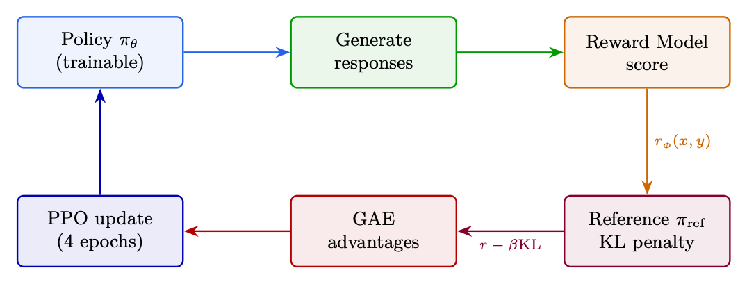
Figure 5.1: PPO end-to-end: from prompt batch through generation, reward scoring, KL computation, advantage estimation, — Figure 5.1:PPO end-to-end: from prompt batch through generation, reward scoring, KL computation, advantage estimation, to clipped policy update. The feedback loop shows the updated policy being used for the next generation step.

PPO manages two distinct parameter states in memory, which share the same neural network topology but hold different weight values during optimization:

Phase 1: Rollout (Data Collection)

During data collection, the agent interacts with the environment for $T$ steps. At each time-step $t$ :

The environment yields the current state/observation $s_{t}$ (for LLMs: prompt + tokens generated so far).
State $s_{t}$ is passed through the current network snapshot ( $\theta_{\text{old}}$ ).
The network outputs raw unnormalized values — logits $z_{\text{old}}$ — a vector of size $|V|$ (vocabulary size 32K–128K).
Probabilities are computed via Softmax: $\boxed{P(a\mid s_{t})=\text{Softmax}(z_{\text{old}})=\frac{\exp(z_{\text{old},a})}{\sum_{j=1}^{|V|}\exp(z_{\text{old},j})}}$ (5.14)
An action $a_{t}$ (next token) is sampled from $P(a\mid s_{t})$ , and the transition tuple $\langle s_{t},a_{t},r_{t},s_{t+1}\rangle$ along with $\log\pi_{\theta_{\text{old}}}(a_{t}\mid s_{t})$ is stored in the rollout buffer.

Phase 2: Optimization Loop (Mini-Batch Updates)

Once the rollout buffer is full, PPO runs $K$ epochs (typically 3–10) over mini-batches. For every gradient step, logits are generated for both policies using the stored state $s_{t}$ :

Old Policy Evaluation (frozen):

z_{\text{old}}=f(s_{t};\theta_{\text{old}})\quad\longrightarrow\quad\log\pi_{\theta_{\text{old}}}(a_{t}\mid s_{t})=\text{LogSoftmax}(z_{\text{old}})[a_{t}]

(5.15)

Implementation shortcut: reuse the stored scalar from rollout instead of re-computing.

Live Policy Evaluation (updating):

z_{\text{new}}=f(s_{t};\theta)\quad\longrightarrow\quad\log\pi_{\theta}(a_{t}\mid s_{t})=\text{LogSoftmax}(z_{\text{new}})[a_{t}]

(5.16)

Because $\theta$ updates after every mini-batch gradient step, $z_{\text{new}}$ changes continuously throughout the optimization loop, whereas $z_{\text{old}}$ remains perfectly static.

From Logits to Probability Ratio

The core PPO ratio measures how much more or less likely an action is under the new policy vs the old:

\boxed{r_{t}(\theta)=\frac{\pi_{\theta}(a_{t}\mid s_{t})}{\pi_{\theta_{\text{old}}}(a_{t}\mid s_{t})}}

(5.17)

To avoid catastrophic numerical underflow/overflow from dividing raw probabilities, the calculation is performed in log-space:

The ratio is recovered via exponentiation of the difference:

\boxed{r_{t}(\theta)=\exp\!\left(\log\pi_{\theta}(a_{t}\mid s_{t})-\log\pi_{\theta_{\text{old}}}(a_{t}\mid s_{t})\right)}

(5.20)

This ratio is injected into the PPO clipping objective:

\boxed{\mathcal{L}^{\text{CLIP}}(\theta)=\hat{\mathbb{E}}_{t}\left[\min\!\left(r_{t}(\theta)\hat{A}_{t},\;\text{clip}(r_{t}(\theta),\,1{-}\epsilon,\,1{+}\epsilon)\,\hat{A}_{t}\right)\right]}

(5.21)

The PPO Weight Lifecycle

Phase	Live $\theta$	Old $\theta_{\text{old}}$	Ratio $r_{t}(\theta)$
1. Rollout Start	Active copy	Same active copy	Always $1.0$ (by identity)
2. Batch Step 1	Computes gradients	Frozen	$1.0$ (initial step)
3. Batch Step $N$	Modifying ( $\theta\neq\theta_{\text{old}}$ )	Frozen	Deviates from $1.0$ (e.g., $1.06$ , $0.94$ )
4. Clipping Active	Bounded by $\epsilon$	Frozen	Trapped at bound ( $1\pm\epsilon$ )
5. Optimization End	Highly optimized	Discarded	N/A
6. Next Cycle	$\theta\rightarrow\theta_{\text{old}}$	Receives fresh $\theta$	Resets back to $1.0$

Table 5.1:Evolution of $\theta$ and $\theta_{\text{old}}$ across PPO training phases.

Continuous Action Spaces Extension

For continuous action spaces (not typical for LLMs, but important for robotics RL), the network outputs distribution parameters instead of discrete logits:

Predicted mean vector $\mu$
Predicted standard deviation vector $\sigma$

Log-probabilities are computed via the Gaussian log-PDF:

\boxed{\log\pi(a_{t}\mid s_{t})=-\frac{1}{2}\left(\frac{a_{t}-\mu}{\sigma}\right)^{\!2}-\log(\sigma)-\frac{1}{2}\log(2\pi)}

(5.22)

The ratio $r_{t}(\theta)=\exp(\log\pi_{\theta}-\log\pi_{\theta_{\text{old}}})$ is then computed identically and fed into the same clipping objective.

TRL Implementation

The HuggingFace TRL library [376] provides production-ready implementations of all major RL methods for LLMs.

from trl import PPOConfig, PPOTrainer, AutoModelForCausalLMWithValueHead
from transformers import AutoTokenizer
from peft import LoraConfig
 
# Model setup
model = AutoModelForCausalLMWithValueHead.from_pretrained(
    "meta-llama/Llama-3.1-8B-Instruct",
    torch_dtype=torch.bfloat16, device_map="auto",
    peft_config=LoraConfig(r=64, lora_alpha=16, target_modules=["q_proj","v_proj","k_proj","o_proj"])
)
tokenizer = AutoTokenizer.from_pretrained("meta-llama/Llama-3.1-8B-Instruct")
 
# PPO config with all critical hyperparameters
ppo_config = PPOConfig(
    learning_rate=1.5e-6,        # Low LR for stability
    batch_size=128,              # Prompts per step
    mini_batch_size=16,          # Gradient accumulation unit
    ppo_epochs=4,                # Epochs per batch (reuse data)
    gamma=1.0,                   # No discounting (single turn)
    lam=0.95,                    # GAE lambda
    cliprange=0.2,               # PPO epsilon
    cliprange_value=0.2,         # Value function clipping
    vf_coef=0.1,                 # Value loss coefficient
    init_kl_coef=0.05,           # Initial KL penalty
    target_kl=6.0,               # Adaptive KL target
    whiten_rewards=True,         # Normalize advantages
    gradient_accumulation_steps=4,
    max_grad_norm=1.0,
)
 
ppo_trainer = PPOTrainer(config=ppo_config, model=model, tokenizer=tokenizer,
    dataset=prompt_dataset, data_collator=collator)
 
# Training loop
for batch in ppo_trainer.dataloader:
    # 1. Generate responses
    query_tensors = batch["input_ids"]
    response_tensors = ppo_trainer.generate(
        query_tensors, max_new_tokens=512, temperature=0.7, top_p=0.9, do_sample=True
    )
    # 2. Score with reward model
    texts = [tokenizer.decode(r, skip_special_tokens=True) for r in response_tensors]
    rewards = [torch.tensor(reward_model.score(q, r)) for q, r in zip(batch["query"], texts)]
    # 3. PPO update (handles KL, GAE, clipping internally)
    stats = ppo_trainer.step(query_tensors, response_tensors, rewards)
    # Monitor: stats["ppo/mean_scores"], stats["ppo/policy/approx_kl"]

Critical Hyperparameters

ParameterTypicalEffect of Getting It Wrongcliprange0.2Too low: no learning. Too high: instability.init_kl_coef0.01–0.1Too low: reward hacking. Too high: stuck at SFT.target_kl4–8Adaptive controller target. Lower = conservative.ppo_epochs4Too many: overfits to batch. Too few: wastes gen compute.learning_rate $1{-}5\times 10^{-6}$ Too high: catastrophic forgetting.batch_size64–256Larger = smoother gradients, more gen compute.temperature0.7–1.0Lower: less exploration. Higher: noisier advantages.